Not just hopefully, its truly working

I am 90% certain that now I am onto just computing through clusters. Everything seems to be working very well. The parameters are great visual fits. Some masses I am getting almost too accurately (.05 solar masses), some not very accurately (1 solar mass), but that seems determined by the accuracy of the age determination, which relies on the photometric error and quality of the data.

Most of the time I know the mass to about +- .2 solar masses.

Q Correlation fixed

So I first thought it would be really tricky to factor in the correlation between b and v for a given q. Thanks to a nice shower, I have now realized it actually reduces the number of calculations I would need to do each round. I pulled the probability of error in V (B respectively) from a vector of values. I have merely changed that vector into a matrix. The element I choose from the matrix is determined by both the error in V and the error in B. Simple. Problem solved... hopefully

Bit more confusing than i hoped

Partly I have not accomplished a lot this week because of the fickle nature of my program. When I first got the griding working, it looked perfect. Then I went to sleep and woke up the next day to start applying it.

For clusters with larger photometric errors, younger ages were always more favorable according to an exponential like distribution. The way I factor in the binary distribution allows for the program to think a red giant is a really noisy main sequence star. The blue error and visual error are uncorrelated in my program. For an actual binary star, it would increase in magnitude for both filters, not just one. A binary companion would not provide a blue magnitude boost while not emitting any visual light.

Thinking about it now, I should actually take that correlation into account when computing probabilities somehow. Might be tricky though. I would have to calculate the most likely q for each star, then compute the probability for each star. This would slow things down a lot. I would get some useful binary statistics out of it though.

From these problems, I've decided to run both methods on each cluster and use the one which seems more reasonable.

To control the Cross Entropy/ Bootstrapping Method, I am going to take prior information more into account. If part of the distribution is not a remotely conceivable visual fit, I will eliminate it. Also, sometimes a point does not seem grouped in the overall distribution and appears as some background noise. So to eliminate that I am discrediting all ages that only have one hit.

I am also going to start taking prior information into account when calculating the mass probability distribution. I know the star is a red giant and not a really noisy main sequence star.

The tech people finally figured out why I didn't have access to gio (separate account), and as gio is many times faster I can progress much more rapidly now. Hopefully. Always only hopefully.

I feel like this project is chasing me in circles. But I guess I don't know what is the best way until I try many possible ways. There is no simple solution that I can attain on the first try. There is no reason to have expected this to be easily accomplished. These facts are things I conceptually heard before but never truly understood as much as I do now.

PS- If I don't get this all done in a week I'll finish it up at home.

New gridding adventures

To contrast the performance of the Cross Entropy method, I modified it slightly to brute compute on a 30x30x30 parameter grid with solar metalicity. Surprisingly enough, it isn't that much slower. Running times are actually roughly comparable, and the gridding method isn't subject to random noise. I could use the CE method to get an age estimate when there isn't any previous estimate off which to choose my grid, but switch to gridding to get the PDF.

Well, I was getting delta functions again and way too large -log likelihoods. But now writing about this I realized that I was marginalizing over the other parameters before exponenting the -log likelihood. So now its turning out quite nicely.

I guess previous problems put me off the gridding method, but now I see that it is probably the way to go. The one problem is that I can't use U-B data without doing a for-loop to fit for E(U-B). IDL couldn't handle the size of array necessary to account for four variables.

So tomorrow, I will start running everything through this and test the effect of binary percentage. I think I'll start working on my final paper and presentation too while waiting for things to run.

Stellar Oscillations in Planet-hosting Giant Stars

Artie P. Hatzes and Mathias Zechmeister

2008 Proceedings of the Second HELAS International Conference

Hatzes and Zechmeister performed very thorough observations of HD13189, Beta Gem, and Iota Dra, stars with confirmed exo-planets, to better characterize the jitter and oscillation modes of the stars. They compared their results with formulas from Kjeldsen & Bedding, and they were consistent for Beta Gem and Iota Dra, but not for HD13189. The discrepency in HD13189 is thought to arise from the predictive power of Kjeldsen & Bedding's formulas primarily in higher order modes, where HD13189 is pulsating in approximately the second mode. They also mention the possibility of constraining stellar masses based on the properties of oscillation modes.

HD13189 also has a very large scatter of 50 m/s, and its mass is also imprecise to the range of 1-7 solar masses. But it has a predicted jitter amplitude of 500 m/s, it actually smaller than predicted.

Other interesting facts in the article: it took 26 years of observations to confirm the planet around Beta Gem. The mass estimate also started out 2.8, but then it got switched to 1.7.

Stellar Mass Distributions

So now I have a successful code to compute the PDF and CDF for a star's mass in an open cluster. I have uploaded the results for NGC2099 star no 108. It has an expected mass of 1.97 and a 90% confidence level of [1.7 , 2.26], a 0.56 mass range. The mean mass is 0.3 lower than what I roughly had, but WEBDA has an open cluster log age of 8.85, instead of the 9 or so that I got.

So it turns out the mass grid for each parameter set is different, so I had to round to a standard mass grid with 1/30 solar mass intervals in order to marginalize over all the parameters. When multiple points on the old mass grid rounded to the new point, I would then take the average of all the probabilities.

I am actually comtemplating retrying the gridding method using my new additions for binary population, IMF, etc. With a rough enough grid, it might actually be only less than an order of magnitude worse. And it wouldn't be subject to the random pertubations of CE and the underestimation of errors of bootstrapping.

For the next two and a half weeks, I only need to run the procedure through all the clusters and stars, and rework a couple of things in the survey optimization. I also want to determine what would be the most efficient amount of time spent on this survey/ at what time would getting more objects decrease the quality of the objects too much. I wonder what is the overall average rate of planet discovery per telescope time.

Errors and the Bootstrap Method

So, I had to fiddle a little with the normal code again because it started acting up, changing ES parameters I think, and checked to make sure it worked on some other clusters.

Then I wrote a procedure to apply the boostrap method to the Cross Entropy. Shown is the histogram for the age. Interesting how some become just completely wrong. So I fitted for the parameters 50 times, each time having scrambled the residuals.

All this didn't actually turn out as efficiently time wise as I would have hoped, but it works.

Finally SUCCESS

So, I was using the following formula

Prob( star's data | parameters)=Prob(star is member)*Prob(star's data|parameters, is a member) +Prob(star is not member)*Prob(star's data|not a member)

And this is all fine in a theoretical way, but when it comes to programming, the second term is so much larger than the first term that the first term mostly gets rounded out. So now, I just add 1e-307 to the first term to keep from taking the log of zero. And it works!

I still need to do some tweaking of CE parameters to make it most efficient, but it is in essence working. NGC2099 is log t = 8.56, m-M=11.66, E(B-V)=.31, in great agreement with published parameters. YAY!

stupid, stupid little details.

Insuffiently detailed isochrones

So, the reason the -log likelihood wasn't being calculated correctly dealt with the step size in the isochone. The difference between one isochrone point and the next on the main sequence can be several tenths of a magnitude and larger than the photometric error. Therefore this influences the probability. Getting stars near isochrone points is just as important as getting stars on the general shape of the isochrone.

In order to combat this problem, I linearly interpolated between neighboring points to create two new points at one third intervals between the original points. This hopefully will not introduce too much error because of the small range over which I am performing the calculation. I checked the Y2 isochrones, and they had an even worse grid. I may still search for another, better isochrone source.

While it now centers around the predicted age, an actual peak doens't really exist. Seems like there is a minimum -log likelihood value, that cuts of under. This is my next problem to fix.

And congratulations to Mary on a beautiful presentation :)

No Progress

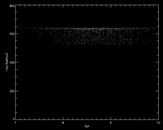
So, I still have not figured out why my program highly favors really young ages and ignores the turn off and red clump. Obviously the Cross Entropy framework is fine since it worked so well for distance moduli, as you can see the plot of all moduli from the parameters sets versus the corresponding -log likelihood. Yet a lower age always allows a better fit?

I created fake stardata just out of the points from an isochrone, and then it didn't go to zero, but it still undershot. I do not understand what that test might suggest.

Anyway, I believe it is NOT as a result of the membership probability, or the CE framework, the IMF, how I am marginalizing over mass, a mess up in dimensions, how I read in the grid, the few outliers, or how I'm weighing the average of the best points by 1/-log likelihood,

TARGET GOAL REACHED and code still frustrating

I have listed 100 targets, my goal.

Well, I should actually cut a few of those out for being too far south, but I'm basically there. How far south can I go?

Also, my code does not quickly send the cluster parameters to zero after a few iterations anymore. Typo in calculating the averages. Also, I can't use ASCC-2.5 data. Even though Kharchenko et al 2005 did, I don't see actual cluster like features on the CMD.
Though those mistakes are eliminated, I can't seem to get the proper values. The main sequence gets fit quite nicely, but it completely ignores the turn-off and the red clump. Especially since NGC2099 has a nicely defined red clump, what happens when it is sparse or non-existent?

WEBDA mistake?

So the age quoted for NGC2204 in WEBDA is completely wrong. It doesn't fit the data. The most recently published value, which does fit the data, is different by almost one entire Giga-year.

Also, their UBV color magnitude diagram is different from the one the data gives.

This is not a cluster I could use, but I think I should still report the inconsistencies. Not sure how though.

Also for NGC2818, the photoelectric data is mildly consistent with the parameters, but the CCD is just not. Where I found published parameters, they agreed with WEBDA's values that don't fit.

Membership Determination Problems

So the majority of today has been trying to get my membership probability calculating program to work. It's now giving resonable numbers, though I believe I'm actually fundamentally misunderstanding basic statistics and completely messing up.

So I'm using distance from cluster center, and RA/ DEC proper motions as given by ASCC-2.5. So, the probability of a data is just the value of the Gaussian at that point. But when I see membership probabilities in WEBDA, they seem much higher. How do they get a 98% membership probability if the peak 1/sqrt(2pi)*sigma is less than that. And other places speak of 67% chance as a 1-sigma confidence interval. Being 1-sigma away from the mean doesn't mean the value of the Gaussian is 67%. And doesn't a PDF only start having meaning when you integrate and say the probability of something between two values?

So I was thinking along the integration lines, and started computing the probability by measuring what percentage of the PDF it was better than. Something in the center has 1 and at infinity has zero. Though I guess 1-sigma is then 33% not 67%. I don't know.

Also, how do I bring together three different probability sources. No matter how good a star is, multiplying them, which follows formulaic logic, is going to lower its probability. The new data will confirm that its a good point, but the probability will go down.

I feel like I should understand this stuff.

On the bright side, I started running a basic level of the code earlier when I left Cahill, and will check it in the morning. I only need to decide on the metalicity grid to add that dimension, which should be finished tomorrow. I also want to get a specific book about Cross Entropy from the library to research parameter tuning.

After I finish those details, I need to figure out bootstrapping and implement that. I don't understand bootstrapping yet, but it shouldn't take too long to master. To finish, I will test the program's efficiency. My plans to test efficiency include creating a synthetic cluster and attempting to retrieve input parameters. Also, I want to determine the influence of binary population, use of weights, IMF, smoothing parameters, and isochrones source (Padova etc.) on the output. I plan to finish this all next week and get started on the mass fitting protocol. The mass fitting protocol should be simple when compared to this process.

Finishing those, I only need to run clusters through the code pipeline and get back masses. Clusters with previously unpublished values can also be calculated and possibly included in the survey. I believe I will be able to get the necessary stars.

Oh- and I'm writing my second progress report this weekend.

Small victories and Weighting Plan

I have now created my smeared gauusians and developed a way to import grids into idl variables :)

I have also decided on a plan of action for the "weighting". It served the purpose to decide cluster membership, so I will proceed to take into account cluster membership according to a Bayesian approach.

Let X= parameters of cluster and Prob(member|X) be A

Prob(Data| X )=Prob(D, member | X) + Prob(D, non-member |X)

=Prob(member| X)*Prob(D | member, X) + Prob(non-member|X)*Prob(D | non-member,X)

=A*Prob(D|member,x) + (1-A)/[(Vmax-Vmin)*(Bmax-Bmin)*(Umax-Umin)]

The last step follows from the probability being independent of the parameters and uniform over the parameter space. The size of the parameter space will be determined by the span of the data.

Though adding complication, I will follow a process to determine A similar to that of Kharchenko et al 2005. Solving my problem of uniform data set, I will use ASCC-2.5 data. I may limit that data source to those clusters with distance moduli less than 11 to keep a wider range of main sequence above the 14 magnitude limit. I will model location and proper motion (parrallax for closer clusters too), and determine membership probabilities based of the dispersion in those values.

Eliminating Pre-Conceived Notions

Even though we have errors in only magnitudes and isochrone data in magnitudes, and my code if fact fits in magnitude-magnitude space, for some reason I and many other papers still primarily think and speak of color-magnitude space. I need to change my thought process to focus around magnitude-magnitude (Magnitude^3 when including U) space.

This means the binary fraction also introduces errors in U and B. I am near completing the protocol for computing probabilities accounting for a binary population.

I am also doubtful as to my need to factor in the initial mass function. Does it put unproductive weight on lower stars?

As to the weighting topic, I am trying to determine the Bayesian logic behind assigning a weight. I am thinking the logic behind it deals with the certainty which we believe the star came from the cluster. If a star is in an un-populated region on the CMD and away from the isochrone, the probability quickly drops to zero and is barely effected by changes is the parameters, so it does not have any importance anyway.

I am also trying to understand working with three dimensional arrays to eliminate a for-loop. My brain does not like wrapping itself around what I need to do. I have read some good tutorials and believe I will manage it soon.

Planning A New Cluster Fitting Protocol

By studying a wider array of literature on the subject, I have become aware of multiple systemic errors in my code that need modification and improvements that I could enact. What I had been doing, though not wrong in the simplest sense, was an oversimplification and not representing the full knowledge that we have on the subject.

Therefore I attempt to make these changes:
1. Change to writing in IDL

It can read in the bulk isochrone files so i don't have to input each age individually
2. Use the Cross Entropy and bootstrapping methods
This will allow me to perform 3
3. Take larger and finer time and metallicity grids

4. Use U-B information as well
5. Factor in the probability that each star is a binary
Accomplished by changing the star's distribution function to a smeared Gaussian
6. Weight each star based similar to Mendieros
7. Use one reference source for the data
8. Factor in the Initial Mass Function

Unsure of how to accomplish this... maybe weighting the isochrone points
9. Perform for multiple theoretical isochrone databases to analyze systematic error arising from theoretical underpinnings

After all these, I will test my program using simulated clusters before applying them to the real thing.

Fitting isochrones to open cluster photometric data

Monteiro et al
A&A 2010

Monteiro solved for the parameters of an open cluster using the Cross Entropy method and analyzed the errors using the bootstrap method, instead of direct computation of the direct tau-squared space. This allows for a much larger grid. Right now, I limit my space to those near the published values.

The cross entropy method first randomly draws a certain number of parameters, and evaluates some function S(x) to be minimized at each point The points are ordered and the best N are selected out. These N define a mean and standard deviation around which to normally draw the next set of points. Weighting the mean and standard deviation with those of the previous round allows the process to converge less quickly and avoid local minima.

The function S(x) used to evaluate the quality of a point was the -log likelihood. Like Flannery & Johnson 1982, they use a nearest point estimator, only paying attention to the point which is closest. I believe that the nearby points should be considered as well and the probabilities added. This makes it more favorable for a star to exist in a area with a larger possible mass range, an important factor.

When the compute the probability for one point, they use the same Gaussian distribution I have been using, but also factor in fitting U-B as well, using all available data.

One of the most important topics in the paper dealt with determining which stars to exclude and giving stars weighting factors. The triangle of cluttered background stars near the bottom was completely cut out. The exact point of cutting did not effect the end result significantly. A cluster radius was computed using density given by positions in the image. Background stars outside this radius were excluded.

To compute the weighting factor, each gained a box with 3 sigma on each side. A Gaussian was computed using the mean and standard deviation for B, B-V, and U-B of stars in that box. It also included a term for its radius from the cluster center. This put importance on stars in the densest of the diagram and in the cluster center. The weight of each star was a factor in its probability.

After setting up the process, they performed multiple checks to assess the quality of the program. They created multiple synthetic clusters and checked if they could regain the same values. They took well-studied clusters and cross-referenced their values with those published. They studied the effect that different IMF's and binary % had on the results. IMF did not have an effect, but binary ratio could effect the distance up to 10%, though age remained the same. The technique was largely successful.

They used standard photometric errors (not those intrinsic to the data) as published by Mointinho 2001. They worked of Padova isochrones like the ones I'm using. They also fitted for E(B-V) in the beginning using a color-color diagram and only allowed it to vary 10% from that value. They also isolated data from only one source, and chose those with U-B data as well. They took 100% binary ratio with companions pulled from the same IMF.

Monte Carlo Simulation Summary and Explanation

Conceptual: The Monte Carlo simulation I performed works on a format called simulated annealing. The process mirrors the metallurgy technique to improve the crystalline nature of a metal.

At high temperatures, metal atoms possess too much kinetic energy to settle down into any lattice framework. If they reach a potential energy minimum, they jump right back out again. The structure is completely random. Quickly cooling a metal forces atoms to stop where ever they are, leaving the mostly random state intact. But cooling the metal slowly enough allows atoms to move around to find the lowest potential minimum before they settle for good. After some cooling, when they find a potential minimum they could stay there, but temperature could allow them increase in potential energy. This increase could allow them to travel to a global minimum instead of a mere local minimum.

So our test point randomly explores the survey quality function (I'm not sure if what I used could be considered a likelihood function) acting like a atom exploring a potential energy function. Our test point starts hot, with a high probability of accepting even an unfavorable new point during its random walk. During the cooling timescale, it steadily calms its jumpy nature and hones in on a minimum.

Practical: To best understand the actual implementation, I will walk through the computing steps.

After receiving a starting point, it randomly permutes both the number of observations and the number of stars which would characterize a survey. Safety measures must be implemented to keep those parameters from exceeding possible bounds and ending the simulation.
In the beginning I imported an array of the magnitudes. Given the magnitudes of the brightest required number of stars, 60 hours of observing time, and each star needing to get the specific number of observations, the lowest instrument noise is calculated. Stellar jitter for each specific star is randomly pulled from a Gaussian centered at 15m/s with a standard deviation of 3 m/s. Stellar jitter and instrument error are added in quadrature.

Next, the parameters are sent into a survey function. 100 simulated surveys are run and the average number of planets discovered is returned. Within a survey, a star is randomly given a planet with a probability equal to .07 times its mass (the masses were also imported earlier on). The planet's properties are randomly selected from a distribution modeled on available data for intermediate mass stars. Each star receives n observations at times randomly pulled from the possible time vector. Three possible days exist per month over a 36 month period. "Observations" consist of calculating the radial velocity due to the planet and adding Gaussian jitter according to the noise. A planet is considered detected if the RMS of the observations is three times greater than the noise level.

Once back in the main simulation, the new set of parameters is kept if either

A. the number of planets produced is greater than that before
B. A uniformly randomly generated number is less than exp( - diff in planets/ Energy)

Hence at high energies, there exists a high chance of excepting the number, and at low energies the probability shrinks. I set the energy timescale to a decaying exponential according to advice on the internet. The energy starts at 20, and each step the energy decreases by 0.2%. I selected the numbers to start very jumpy and end very cold.

If the point is accepted, it is returned to a file.
This process is repeated 5000 times.

(And I just learned a good deal about making aesthetic graphs in MATLAB)

Why still a delta function PDF?

So...
Since the mass is still way too precise, I decided to move backward and look at the cluster fitting parameters. They turn out to be extremely precise too. Way too precise.

So, I went back and looked at the fitting paper that I read and I section that didn't make since before now makes since and I may be greatly wrong as to my process. They take the original isochrone, populate the HR diagram with many,many stars from this isochrone according to the initial mass function, and make a certain percentage of them unseen binaries according to some other distribution function. This creates a density on the HR diagram that is used to compute probabilities of a data point from that isochrone. Though the code would not be incredibly hard to write, it would be computationally difficult and greatly increase the time necessary for one cluster. Is that necessary and where I am going wrong?

Before I get too overwhelmed and confused, I think I'll try this on another cluster to compare results.

Better than a delta function PDF?

So I found an error in my code (I was dividing by the standard deviation in two separate places). The peak now does not move with a changing RMS.

And the error bounds are slightly better being twice as large, .002 solar masses instead of .001 ...

Survey Update
Stars:70
Clusters:24

All clusters with NGC# < 2287 have been completely rechecked for any hint of viability

Delta Function PDF?

So I am improving my cluster parameters fitting function, and creating my mass fittingfunction, and have a feeling something is wrong. All the code seems right. The cluster parameters returned visually fit the data well. The mass returned is within .1 of the rough distance only mass approximation. But the PDF for the mass is a delta function. I'm pretty sure we can't know the mass to a greater precision than .001 solar masses.

Later on, I have discovered that the PDF and even the maximum is highly dependent on the error. The RMS quoted for the star is .003, but MATLAB won't handle the extremely small probabilities that result from that. And obviously 67% of the bright stars are not .003 within a predicted isochrone. So I used .03, which gives the delta at 2.227, but I move it to .3, and it changes and moves the maximum to 2.5 (part of the loop that it obviously doesn't belong to).

I believe astrophysical properties, and not instrumentation, determine the majority of the error. Thus, I will fit all the clusters, and determine the error from tabulating the distribution of stars around their isochrones.

Note: I just eliminated fainter data since it included many background stars not even close to being on the main sequence, and I used CCD data.

Survey Update
Stars:64
Clusters: 20

Two Sato et al papers

Sato et al. is a group of scientists in Japan looking at evolved intermediate mass stars, and discuss six new discoveries over two papers. They also include some interesting speculation as to the less than 0.6 AU planet desert and the apparent lack of a metallicity correlation for intermediate mass stars. For post-red giant tip red giants, they could have actually engulfed the planets, but that does not explain the lack of inner planets around sub-giant stars. A different formation mechanism may be at work.

Important for my research, they include jitter values. As I previously assumed, the jitter seemed around 15 m/s. 10 m/s was the norm for the sub-giants they used, but the full red giants had more jitter. They had one at 25 m/s, but it displayed chromosphere activity in the Ca II & K line analysis.

BEST RESULTS!!!

Pretty sure this is correct now.....

4 observations each of 100 stars gives 18.82 planets

Seems reasonable, and should be returning right about how many I assigned :)

Better Results

So when I left last night I set the Monte Carlo simulated annealing program to run for 5000 iterations instead of 1000. Now the optimum is even better
.....
6 observations of 96 stars gives 10.82 planets.

I did get "arithmetic error: floating underflow" and "arithmetic error: Floating illegal operand", but the results seem legitimate.

Except, yeah, none of this actually practically works. I didn't set a lower limit on Signal to Noise, so its at a completely unpractical low level. Um... I'll write in a lower limit and run it again. That's probably why its actually returning 10% planets instead of 20%.

Except, yeah, I just spent an hour or so trying to figure out what was wrong with my instrument noise formula, and I had .01 as a constant instead of .002. Yeah, who knows how many times I recalculated it and kept getting it wrong. Works now :) Will run another simulation of 5000 now and see what happens :)

RESULTS!!!!!!!!!!!!!! :) :) :) :) :) :) :) :) :) :) :) :) :)

FINALLY!!!!!!!!!!!
THE MONTE CARLO SIMULATION RETURNED LEGITIMATE RESULTS!!!! MORE CAPSLOCK!!!!!!

It ended on.......
drumroll......

26 observations of 68 stars yielding an average of 6.2 planets.

Actually a couple earlier 24 observations of 68 stars yielded 7.02 planets, which is the best of the 985 accepted new points. I think I need to tighten the acceptance probability at the end and also run more iterations, since it still jumped around a bit near the end. Also, 986 times it accepted new points out of the thousand iterations? Definitely tightening acceptance criterion/ running more iterations.

I'll run it for 5000 iterations right now, and check back after dinner!!!!!!

A Jupiter-Mass Companion to a Solar Mass Star

Queloz and Mayor 1995

Annoyed as I was at the de-bugging process, I decided to take a break while my Monte-Carlo code ran and read Queloz and Mayor's historic Nature paper about 51 Pegasi b.

The paper is actually quite exciting. These five little pages were the start of this entire field. The "intensive observations during eight consecutive nights" sounds very exciting for all the technical language in the paper. I can only imagine what it might have felt like to be at that discovery.

The tone of the paper is different then other planet papers I've read. They definitely expected a lot of opposition, which I guess they got. Each objection seems to be carefully thought out and analyzed. Now I assume there is a specific process to eliminate all sources of mistakes, but they got to come up with it all themselves. Quite fun.

In the details, I liked learning that giant pulsating stars pulsate simultaneously in many short-period modes. I guess that does make sense considering what I'm working through in Carroll and Ostlie on stellar pulsation.

Some Results! Statistical distinctiveness

disclaimer: using 30 random observations over 1000 days and constant 2.5 solar mass

0.18 planeticity (predicted for 2.5 mass solar metallicity stars) is inconsistent with zero above 20 sampled stars. :) The prediction is 3.58 planets with 1.63 standard deviation. Great!

But, only at 100 stars does 0.18 planeticity start being inconsistent with 0.08 planeticity. I think it will only be by combining this survey with other work that we will be able to say for sure that intermediate mass stars do have a larger planeticity :( As shown in the graph, a survey drawn from the 18% distribution could easily fall in the 8% distribution area.
On the bright side, my average mass might end up being greater than 2.5, so the planeticity will be greater and it will be easier to tell them apart. Also, standard low mass stars are populated by a different population of planets which would probably be unobservable around intermediate mass red giants. 100 good targets will probably be an upper limit for how many good targets I can find (maybe), and I don't now how time will limit it.

I did approximate the multiple survey standard deviation as coming from a Gaussian, which might be wrong. It kinda looks triangular shaped. I don't know how to save IDL graphs so I can't really show an example in the blog. Anyway, I used the criterion:
| nplanets(0.18)- nplanets(0.08)| > 2 * sqrt( sigma(0.18)^2+ sigma(0.08)^2 )
to determine distinctiveness.
Both the average and the standard deviations were pulled from 100 trial surveys.

So the assigning planet program has been altered to actually pull from the mass law (Making my Own Distribution Functions) and a uniform distribution for radius over 0.6 to 3 AU. I struggled with algebraic manipulation and units for a while, but now it works quite fine. Also, returnability is calculated by RMS > 3 *noise instead of seeing if rv_fit_mp returns the same parameters. This is much more rapid and efficient. 4 seconds for 100 surveys, so I can run 100 surveys per step and still get many more steps in. Also, since we probably won't actually have incredibly much control over observing schedule beyond how many observations, observing dates are now completely randomized.

Goals for tomorrow:
1. import in array of magnitudes and masses from current available stars
2. calculate noise
3. Make sure MC parameters and time scales are good
3. Start running MC program AND SEE WHAT HAPPENS!!!!

Turtle wins the race? eventually...

I tried reading some books in the library on the Monte Carlo method, trying to find descriptions of simulated annealing. While I didn't understand a lot of it, I did get:
the probability of accepting a worse point is e^(-diff/temperature parameter). that helped.

I have also added in a permutation of the time each round. The code also prints the results each round.

I have also added in the "temperature" that controls acceptance of worse results. Some simulated annealing tutorial said Tnew= alpha * Told was a common annealing schedule, so I decided to adopt that. I would like to research that choice a bit more though. I set alpha as .998 so that it could still move up half way through a 1000 long run, but probably not accept anything near the end.

I decided a 1000 long run based on time. One survey takes about 15 seconds. If I average five surveys per point, then leave about 15 seconds to calculate new point, etc., then 1000 iterations would take 21 hours. I'd like to get it more efficient than that, but I don't know how.

I still need to calculate noise. I also need to restrict time to under 10 hours per semester some how. I think I'll need to keep the time from having two of the same dates some how too.
At least my to-do list is slowly shrinking. I still am trying to read some difficult papers/ books on this subject and experiment optimization.

One paper I'm reading is talking about optimizing future optimizations after 3 or more velocities have been taken. If I could set up that framework now, I'd like to try to implement that into the latter part of the survey if at all possible.


Survey Update
one 9th mag, 2.82 solar mass star in NGC2527 could be added, but SIMBAD doesn't call it a "star in a cluster" like most other stars in clusters

PROGRESS!, well sort of....

Even though I still don't understand much of the papers and will continue to wade through them to understand optimum experimental design (involving completely new ideas like Shannon information and Utility functions), I did manage to make some progress on my Monte Carlo code yesterday. I read in Ford 2008 that he just used a Jeffrey's prior P(x)=1/x, since this represents maximum ignorance about the scaling of a parameter. So I adopted a Jeffry's prior to period and velocity semi-amplitude. I added a uniform distribution for eccentricity, though I want to figure out something better than that. I do not know if a Jeffrey's prior would be right for eccentricity since it is not a scaling.

I have finished (other than the concerns expressed above) writing a "Survey" program and all the things inside it, and am working on the actual body of the Monte Carlo code. That is the progress part of yesterday. I have multiple problems that I am trying to figure out in this. First, the neighbor function/ getting each new point.

Time presents the worst problems. The way I have it right now, time gets changed with the number of observations. Number of observations goes down, dates get randomly eliminated. Number of observations goes up, dates get randomly added. I don't like the connection between optimizing both parameters. Also, it doesn't factor in not being able to observe certain objects for parts of the year. And its the same for all stars. And I have no safeties in place to protect from getting two of the same times into the time vector. And I have no constraints on having time in each semester.

Second problem is noise. Firstly, its dependent on what i do for time above. Second, when I add more stars, I'll have to include dimmer stars, and the average exposure time goes up for the same signal to noise ratio. Do I need to include that and I how do I do so efficiently? Another problem, I do not know how to translate from signal to noise ratio to instrumental uncertainty in m/s.

In the overall category, do I just change one parameter at a time, or all every iteration?

Even though I know the overall theory of the method, I don't actually know how to accomplish specific parts. For example, how should I change the probability acceptance parameter with number of iterations? Does the probability acceptance depend linearly on difference in planets between two points?

Also, do I need to be concerned about efficiency? Running one survey of 100 stars takes me about a minute to run. If I run ten thousand steps in the MC method, that not only includes running the survey each but calculating each parameter to input into the survey, that is a very long time. I don't understand why a survey is an entire minute. Probably stupid FOR loop that I can't eliminate.

Though I am definitely challenged on this problem, I feel like I am learning a lot and gaining an extremely valuable skill. Back to paper reading :)

Survey Update
Two ninth magnitude 3 solar mass stars in NGC2458 have been added. Five others in the same cluster were eliminated for one reason or another.

Nevermind the meaningless blather

So, after trying so hard to figure out the distribution functions, I realized this:

My program could accomplish one of two goals:
1. Tell us what we are going to see
2. Tell us how efficient we will be at detecting what is actually there

If I wanted to predict what the survey will return, I would need the distribution functions like I have been trying, but if I change the goal to merely assess the efficiency of the survey, I should just use a uniform distribution function. That way I can tell how the distribution function changes after experiencing the noise and detection. Maybe later I may run the simulations to predict what we will actually see, but for now I will continue writing my code the simpler way.

Later: Meh, that itself was just substance-less blather... If I am just going for efficiency, then the code will probably just tell me to look at a few things really well. Number of planets is the one way to strike a trade off between efficiency and actually managing to detect a wide number of planets. How would I factor size of sample in to Goal 2?

Further complicating the Goal 1 way to go about things, the distributions that I got yesterday were post-biasing. I need a pre-biasing distribution so I can then bias it and see what happens. But I don't know the parameters of each individual survey to get a "bias surface" to un-bias the surveys.
I don't even know if my weird concept of a "bias surface" exists. It would give the percent observed out of percent present. So simple conversion from the post-biasing distribution function would give the pre-bias distribution surface. Probably requires many more data points than those available.

OH OH!!! Just found paper on survey optimization. Hopefully that will solve my problems.

Survey Update
M44: 1 new red subgiant at 6.68 mag and 2.2 solar masses (4 others eliminated)
NGC6404: 4 9th magnitude possibilities

Making my Own Distribution Functions

The closest thing I found to describing the distribution functions for mass and period around intermediate mass stars was Bowler et al, which only said what the distribution function was not. Therefore, I decided to take matters into my own hands and examine the periods and masses for all stars with masses greater than 1.5 solar masses.

For the 39 data points, the first thing I saw was that mass was mostly a power law. Two lower mass planets at .6 and 1.2 Jupiter masses I ignored, since there were several 1.6 masses with it decaying from there. When I had 1.59 Jupiter masses as the xmin, it fit quite nicely, see figure. I would like to study this more and actually mathematically find the optimum xmin, not this guessing that I did.
Mass Distribution Function:
P(x)=1.3917*x^(-1.9118)


Now the semi-major axis (which translates to period) is more complicated and more sketchy approximation. I threw out the direct imaging stars (Beta Pic, Formalhaut, HR8799) since those were at massively larger semi-major axes and no doubt coming from different distributions. The planet desert less than 0.6 AU was definitely obvious, and planets also seemed to pile up right outside the 0.6 AU boundary. After taking out the 0.6 AU pile-up, the rest of the data points looked Gaussian to me, so I fit them with a Gaussian.
Non-Pile-Up Semi-Major Axis Parameters
Mean- 1.6772 AU
Standard Deviation:0.5149

Retired A Stars And Their Companions. III. Comparing The Mass-Period Distributions Of Planets Around A-Type Stars And Sun-Like Stars

Bowler et al.
The Astrophysical Journal. January 20, 2010

After the introduction and background about many interesting things I need to read more about later, Bowler et al gives updated information about the five stars already shown to possess planets in a 159 star survey. They applied a Bayesian model comparison test to decide whether or not to add in a constant acceleration due to a binary companion (BIC=-2 ln(Lmax) + k ln(N), lower BIC preferred). Parameter uncertainties were estimated using a Markov Chain Monte Carlo algorithm. Even though I understand what they wrote as the process, I am unsure of how they get the actual uncertainties from the chain of steps. Lomb-Scargle periodograms were used to search for additional short-period companions. They also studied all five stars with photometry over an extended time period to tell if the periodicity was a result of stellar activity or if the planet transited.

One of the most interesting parts of the paper for me was when they discussed the Detection Limits. They synthesized fake orbits and determined the highest K that would be detectable with the given noise. In addition to testing the null planets, they tested those with planets for additional ones. Even though they said they could detect less than Saturn mass planets closer in, most of the noise was from the star so detection could not improve much more. The only chance of finding Neptune sized planets would be from transits or micro lensing. Even with the noise, the finding of higher mass planets was probably the result of a real trend.

For this small sample of stars, they compared the statistics to those for stellar-type stars. Approximately 24% of the stars have planets, consistent with other predictions to more planets around higher mass stars. They also tested whether or not the planets could be drawn from the same mass, period distribution as sun-like stars. When including planet occurrence rates, it was less than a 10^-5 probability that they were the same. Even when they accepted different planet occurrence rates, they ruled out them being drawn from the same mass-period distribution with confidence over 4 sigma. Even though they had too few data points to actually find the parameters, they did rule out several regions of the parameter space. There is also a low eccentricity trend for planets around IM subgiants that differs with normal stars.

Extrasolar planets around intermediate mass stars

A P Hatzes
Phys. Scr. 2008

Hatzes begins by reasserting the possibility of a planet around Aldeberan, alpha Tauri. It was one of the first prospective planets along with Pollux and Arcturus (Beta Gem and Alpha Boo). Pollux was later confirmed to have a planet, but neither of the others has been confirmed. If Aldrberan had a planet, it would have a 645 day orbit and M sini = 9.5 Jupiter masses.

Solving the problem of not knowing red giant's masses reliably, they calculated Aldeberan's mass using interferometric measurements of the radius and spectroscopic measurements of the surface gravity. Another method that can be used to determine stellar mass is that usually nasty stellar oscillations. Stellar oscillations are still extremely nasty, and Hatzes quoted the oscillation of a fundemental radial mode with intensity of 150m/s and said that giant stars can have intrinsic variability up to 100m/s.

In 2008 when Hatzes wrote this paper, there had been 20 extrasolar planets around giant or sub-giant stars, enough that he analyzed the trends. They exist in a limited range of period from 160-1000 days, with 1000 days appearing probably from the length of contemporary surveys. Inner planets are probably eliminated either by tthe expansion of the star's radius or new instabilities. 60% of the planets had masses over 5 Mjup, in comparison to less than 20% for normal stars. More massive star means more massive planet. He also found that the distribution of orbital eccentricities is independent of stellar mass. As he had fewer data points, he stated that a uniform planeticity-metallicity distribution was consistent with the data and that many of the planet hosting giant stars are actually metal poor.

Still unable to determine what parameters mean

So in attempting to write code to randomly draw out the parameters, I have to know what each parameter is. I am still unable to decide what gamma and dvdt mean in the output of rv_fit_mp and also clueless as to the identity of cmvel and om are for rv_drive. I'm guessing om means omega though.

Still searching through literature to get good distribution functions to use.
Once I get these problems finished though, it should all come together smoothly.

Planning to Plan for the Survey: Optimization

In order to run the survey most efficiently, I need to run Monte Carlo simulations of thousands of potential observing runs to find the best distribution of time, stars, masses, and signal to noise. Compounded with this, if I run the survey most efficiently, what is the probability I will be able to conclude anything from the results?

Monte Carlo method works based on a modification of a sort of random walk. From an initial guess of parameters, a step is randomly generated according to a Gaussian (or other type of) distribution function. The step is automatically excepted if the survey efficiency (or other metric) is higher. If the survey efficiency is lower, then the point is accepted with a probability proportional to the difference is efficiencies and some "temperature". The "temperature" decreases through out the simulation so that the point goes to the nearest extrema at the end of the simulation.

So inside this method, I need to calculate some survey efficiency at each point given the specific set of parameters. This happens by running many, many simulated surveys and either seeing the average number of planets measured or the number of planets measured out of those present. I think the survey should be run for both methods of efficiency measurement.

For each star within a survey, predicted probabilities will govern the random assignment of a planet to a star. If a star has a planet, more predictions will randomly assign the planet a mass and orbit. Noise will be applied to the respective RV curve, and the computer will try to recover the original planet.

While that is the overall picture, right now I need to read through the literature to discover what the theoretical distributions are. Also, I need to figure out how to randomly draw numbers from a power law distribution in IDL. IDL can give out numbers with various Gaussian, Poisson, flat, binomial, etc. distributions, but no power law that I can find. I have a theory about how to convert flat distributions to power law, but I am not entirely certain about it. (Never mind I found randomp which gives a power law distribution)

Literature Background: A Post from Yesterday

Yesterday I got distracted then fell asleep before finishing up after dinner, so here is what I did yesterday:

I read/ scanned papers looking for references to any of my chosen stars that would reveal them to be either a non-member, variable star, or spectroscopic binary. This eliminated many stars, but actually added a bunch as well. For NGC6134, Mermilliod and Mayor were examining twenty red giants, not just the three I had extracted. The CCD data I had been looking at was incomplete, so I found many more red giants when I looked the plain UBV tab in WEBDA. Also, I realized one cluster I thought wasn't up in late July actually was. All the stars in one cluster got eliminated for one reason or another.

I also added a new cluster, NGC2281 with five red giants.

Today I will add at least two two clusters and assign priority numbers for all stars.

Survey Total
Clusters: 12
Stars: 52

Observing List Compiled and Four New Clusters

Part of the morning was involved in a follow up on the photometry of FGD459 from yesterday. The systematic error between my measurements was never completely explained.

I have analyzed four new clusters, yet one needed to be dropped since I forgot to check if it was visible in July. One cluster has a low metallicity of -0.16 which reduces the planeticity, but other aspects of the cluster make it good for the survey. Another cluster's stars have masses of 4.5 solar masses. This is the largest I've analyzed yet by about an entire solar mass. Lovis and Mayor did include stars in this range, so I think they are legitimate to include.

I also transferred all necessary data into an observing list format. To complete this, I also had to calculate exposure times. I am uncertain as to the correctness of my method to calculate exposure time.

The Handbook of CCD Astronomy says that, for high values, the signal to noise ratio is dominated by error from source and is proportional to the square root of the number of pixels received. This follows from the incoming photons having a Poisson distribution. The number of photons is the flux times the exposure time. Flux can be expressed as 10^((m-48.6)/2.5) ergs/sec, with m in the AB system. AB magnitudes are only slightly off from the Johnson system, so I just used the V magnitude listed. The conversion from ergs/sec to photons/sec I just absorbed into the constant of proportionality. These all give the formula
S/N = C * 10^((m-48.6)/5) * sqrt(t)
where C is a constant of 4.4e12 determined from the rule of thumb "A 8th mag star takes 90s to get S/N=200".

I set the signal to noise ratio equal to 90, solved for t, and rounded up to the nearest convenient number. For stars dimmer than 12th mag, this gives times in excess of a thousand seconds. This seems an inefficient use of time, so those clusters should go to lower priority values.

Tomorrow I intend to search through the literature to find any possible problems with the new prospective stars to eliminate variables, non-members, spectroscopic binaries, etc.

Current Survey Total
Stars: 37
Clusters: 11

Stellar Photometry

Most of the trouble with stellar photometry arose from logging on to the right place, getting the data, and opening atv. Once those got worked through (I still do not completely understand the mysteries of how computers choose to operate), the rest of the work was fairly simple repetition. Even though all my values were internally consistent, there was an offset from Mary's results using a different calibration star. We will examine this discrepancy to a greater extent tomorrow.

I have also added a new cluster, NGC 1496, with three stars around 2.4-2.7 solar masses. New total= 24 stars.

I also read a fascinating article in Astronomy magazine about the possibility of viewing exo-zodiacal light. Written by Kuchner and Stark at the Goddard Space Flight Center, they observed 51 Ophiuchi with the Keck Interferometer Nuller and were able to distinguish between an inner ring of an asteroid belt/ exo-zodiacal dust and an outer Kuiper belt like region. They are also running simulations of the interactions of zodiacal dust and a planet. If our optics systems ever improve to the capability of directly imaging an Earth size planet, the zodiacal dust could just wash it out. On the positive side though, the planet may induce perturbations in the dust that might demonstrate the existence of a planet.

And its a small world after all- there was also an news clip about six planets that orbit contrary to the star. Another news short discussed the lack of methane on GJ436b.

Tomorrow I have a goal of collecting at least three new clusters and calculating all the exposure times.

GOOD VALUES RETURNED!!!!!

After much modification, my MATLAB code now returns the following parameters for M37, NGC 2099:
Age= 440 million years
m-M=11.48
E(B-V)=.25
These values are in good agreement with published parameters. Now that I know the place I am looking for better, I tightened my prior and use a finer grid close to the peak.
Even though the PDF's and results look great, it doesn't look as good a visual fit as one could possible be. I may be just that I am paying attention to how well it fits in the red giant area, which is easier to visually judge. Now that everything else is working, I will modify the standard deviation for each star to account for its position and give more weight to red giants and those on the cut off than those on the main sequence.

I first got my code to work before lunch, but after making the age grid finer it stopped working. I somehow managed to not correctly transfer the new array of isochrone values. Other problems I encountered include rounding to zero for the probability and gaining -Inf for tau squared (solved by adding a very small positive number) and the mysterious Nan 's (eliminated by deleting Nan 's that somehow showed up in my star data). I took out stars obviously not on the isochrone from the data set as well.

Today I also learned that the UBV measurements taken by CCD cameras are on a different link than plain UBV from photographs. Hence I need to change the data I have been working with for all the clusters. It probably does not change the preliminary mass estimates much, but for fitting the cluster later I will need to use the CCD data, since it is more accurate.

I also need to study whether or not it is possible to fit for metallicity. Metallicity does slightly change the isochrone, so I need to determine whether or not it is discernible in a fit.

I have also added three new stars in NGC 6134 at mass 2.14 solar masses. This brings the total to 21 viable stars. For the next few days I will set aside the fitting to focus on getting more stars and calculating priorities and exposure times.

C++ Code

Today I wrote code in C++ to see if it performed differently then what I was doing in matlab. I actually took more time to compute. I believe this is because it not only has to go through the large arrays that are getting imputed, but perform the marginalization as well before I can get data out. I ended up having to just modify my arrays in excel to add brackets and commas and then copy and paste them directly into the code since I could not figure out how to read a vector let alone a two dimensional array into C++ code.
After marginalizing to get a least squares for both time and distance modulus, they were both disparate from the published data and what looks like a good fit. So I have the code, and it computes, but it needs work still.

HR fitting for three parameters and new cluster

I have chosen two new stars in NGC 1528. They are both completely cluster members and around mass 3.1 solar masses. They have unidentified metalicities.

In the arena of chosen stars, I need to find metallicities for more of the clusters, or figure out how to calculate it. I also need to figure out how to calculate necessary exposure times. I want to conceptually work through the process of figuring it out instead of just looking it up, so that will take some thinking. I will continue to add new clusters to the list.

I also worked on extending the least squares fitting to cover distance, age, and reddening. Yesterday I managed to correct my distance fitting mechanism. What I had been doing previously was ignoring algebraic rules and I redid the code correctly and it worked very well. Today I devised a way to compile many age variables into one multidimensional array to use in the fitting process. This allowed me to successfully fit for both distance and age when keeping reddening fixed at the know value of 0.227 . Sadly when I extended it to cover all three variables, distance, age, and reddening, it didn't work. Age just went to the upper limit and reddening was off from the previously stated value significantly as well. Just looking at the plot showed it to be wrong as well.

I marginalized over the parameters in tau squared space, and the peak the code was returning for reddening was not the peak that the plot showed. I don't know what is going on. Age was just an increasing line, but somehow distance still worked quite well. I need to figure out why this it not working. I believe the outliers may somehow be throwing it off, so I need to work a process to account for them into my code.

This is getting to take quite some time to compute, with 11 ages, and 100 for each reddening and distance, with many computations at each combination. To speed things up and hopefully get a code that works, I intend to write a C++ code to fit HR diagrams. Sadly, I do not know how to compile and run the code on my computer since I learned on a fully set up linux computer. So I need to figure that out and write the code. I also need to figure out how to import the multidimensional age array into the C++ code.

Likelihood fitting of distance modulus

I have begun writing a Matlab code to compute the distance modulus, reddening, and age of a cluster through Bayesian statistics. As a first step, I am keeping the proper age and fitting only for distance modulus with cluster NGC 752. For a range of distances around the proper value, I computed the tau squared of the fit, the -2 sum of the logs of the probabilities. Right now I am doing this with two for loops, one for each distance and one for each star, but when I get the code better I wish to use only matrix manipulation, since Matlab is optimized for working with matrices.

After correcting a few errors, I did manage to get a plot which looks right and gives back an answer somewhere in the ball park. I get a distance modulus of 7.36. The actual distance modulus is 8.18 and I can see just looking at the graph that 7.36 is too low. This may be occuring from a line of stars to the right of the main sequence and below the red giant area. Moving downward gets them, out in the middle of no where, closer to the sequence.

My next steps involve getting rid of the for loops, figuring out exactly why the fit is bad, and then working in fitting for age as well.

PDFs, CDFs, and two new clusters

I have added two new clusters to my list, NGC 1664 and NGC 6940, with an assortment of stars in each. I found a cluster that is potentially quite usable, but no one else had an age estimate, so I will work with that after constructing my CMD fitting procedure.

Even though I will fit the masses properly after I have derived my own properties for the clusters, I wrote the program to compute the probability distribution function (PDF) and cumulative distribution function (CDF) for a star given an isochrone. It involves calculating the probability of a given location in the star's Gaussian distribution on the isochrone. For each part of the isochrone, I break it into a certain distance away in the sigma v direction (vertical) and sigma b direction (slope 1) from the star. Each distance is then divided by the respective standard deviations and I take the square root of the sum of the squares. This is the (data - fit)/sigma that goes into the Gaussian equation.
The CDF is merely the integral of the PDF. The PDF is normalized.

The hardest part of this process is actually tracking down the original source of the UBV values to arrive at the error of U and V. Some of the sources are old or have moved around, making it either difficult or impossible to find, so I only managed to compute this for two stars.

A Maximum Likelihood Method for Fitting Color Magnitude Diagrams

In their paper, Naylor and Jeffries presented a method of fitting clusters to an isochrone in a color- magnitude diagram using Bayesian statistics in such a way as to have numerical backing for a fit and to get useful error bounds. For each star, they multiply the star’s Gaussian distribution together with the density of the isochrone, then integrating over all space to obtain the probability that the star came from that isochrone. Tau squared, a very similar quantity to chi squared, is negative two times the sum of the logarithms of the probabilities. A good isochrone fit minimizes tau squared. Minimizing tau squared is the same as maximizing the likelihood that the data came from the given isochrone, since tau squared is a modification of the log of the likelihood. The likelihood of a fit given the data is proportional to the likelihood of the data given the fit by Bayes’s Theorem, so maximizing one is maximizing the other.

Past this theory, several additional factors enter into actual computation. For example, one standardizes the number of stars per magnitude range so that the initial mass function is not a parameter in the fit. Error bounds were found by a bootstrap method when the cluster was simulated (a set of different inputs according to a Gaussian were inputted and the result examined), and integrating over tau squared space gave error bounds in a real cluster. To account for the interaction between B error and B-V error, the color magnitude diagram must be translated into a magnitude-magnitude diagram to compute the probabilities, yet this only happens for the one step.

They worked this method of fitting both on simulated data sets and an actual cluster, and both agreed with the back of the book answer.

There are still multiple things I do not understand in the paper, but they are more details of implementation and terminology. How is the normalization over magnitude ranges accomplished, and why does that not give unfair wait to higher magnitudes? What is the theta and gradient discussed on the seventh page? Though the paper says the method accounts for binary systems, how does it do that?

4 Clusters Choosen

So I have now chosen four clusters and approximately three stars in each cluster. These clusters are M37, NGC 752, Collinder 350, and Melotte 111 (Coma Berenices). I choose them based on age (old enough to have red giants), quality of UBV data, location in the sky, and not already being in a planet survey.

Starting out, I searched through WEBDA's list to find open clusters with positive declination visible during the summer from Hawaii and having log age > 8.5 . I found that clusters with log age less than 8.5 were usually too young to have red giants.

I plotted the B-V vrs. V for each cluster and used published parameters (either on WEBDA or in papers) to get an approximate fit for each cluster. If things did not work at all or the UBV data was scarce and not clear, I would pass the cluster over.


Once I thought a cluster passed those tests, I choose individual stars to get a rough mass estimate for. Since this is a first rough test, I merely computed which point on the theoretical isochrone was closest to the star distance wise. When I go through after getting my own cluster parameters, I will compute the PDF, by analyzing B-V and V separately with their own standard deviations (not just as distance) and assuming Gaussian distributions. That way I will actually be able to get error bounds as well.

Even though I wanted to get an even mass range, I ended up getting a lot of 2.7 mass stars in M37, Collinder 350, and Melotte 111 with 1.7 mass stars in NGC 752. I need older clusters to get lower mass stars, but most clusters, other than NGC 752 and a few others, have dissipated by 1 Gyr of age.

As a continuation of yesterdays post, it was mostly the one star I was focused on that wasn't working. That particular star still doesn't work, but other stars have been looked up in both SINBAD and Hipparcos. Some stars still do not show in the catalogs, but for several I was able to get a more accurate location, official names, and variability information. Some of the 12 stars I had initially chosen now have to get thrown out for either being spectroscopic binaries or microscopically variable.

Accessing data in different catalogs

I have been studying M37 with the data given by the WEBDA database. Now I am trying to access information on the stars from alternate locations but am having a very difficult time trying to locate the same stars. In a paper I read, they accessed the star's data in the Hipparcos database to determine whether or not the star was variable in the visual range. I wish to make sure the stars I am singling out are not variable, so I am trying to look them up in Hipparcos.

I am working with NGC 2099 star no 195 with RA(2000)=05 52 16.25 and Dec(2000)=+32 36 20.7
When entering the RA and Dec coordinates of the star I get "No data returned!" from Hipparcos.
When searching for the star with SINBAD, I cannot get the same star. I get a similar star given by Cl* NGC2099 J136 which also has the designation NGC2099 195. The 195 similarity suggests they are the same star, but WEBDA gives it a V magnitude of 11.009 and SINDAB gives it 11.27. Also SINBAD has a B-V of .5 where WEBDA has a B-V of .76.
So I am stuck.

A Planet Around the Evolved Intermediate Star HD110014

by Medeiros, Setiawan, Hatzes, Pasquini, Girardi, Udry, Dollinger, and da Silva
Astronomy and Astrophysics 2009

Medieros et. all discovered a 835.477±6.04 day period, Msin i = 11.1(9.5) MJup planet around HD110014. Relevant to my research, HD110014 is an evolved higher mass star, but is not in a cluster. The bracketed value after the quoted mass is a result from not knowing the mass of the sun. After computing the PDF for the mass of the main star by summing over all possible parts of all possible isochrones it could belong to, there is roughly equal probabilities of it being a 1.55 Gyr 1.9Msun star, or a 0.68Gyr 2.5 Msun star. A slightly higher C12/C13 ratio gives weight to the 2.5 Msun solution, but both still exist. The 9.5Mjup solution for the mass arises under treating the star as a 1.9Msun star instead of a 2.5Msun star.

After removing the planet, a 130 day periodicity remains. This may be a result of a planet, but the evidence is not strong enough to convincingly say so. Treating and it as a planet and removing from the residuals eliminates all remaining periodicity in the signal.
In order to determine that the 835 period is not the result of stellar phenomena, they ran several tests. I need to read other papers specifically on the bisector velocity span and CaII H&K emission lines in order to understand them better. They also studied the visual magnitude that came from the Hipparcos data. It was classified as a non-periodic star, and no significant peak appeared in the periodogram at 835 days.

Plotting Theoretical Isochrones and Cluster Data

In order figure out the mass of the stars, I have to fit it to theoretical curves for a range of stellar masses at the same age and metallicity as the cluster.

The website CMD computes all the relevant data for a given age and metallicity, and can also factor in extinction, circumstellar dusk, and returns a file filled with data points over a range of masses. In this file are the Absolute Blue B and Visual V Magnitudes.

The WEBDA database has data on each star for a given open cluster. In this I can get the relative B and V magnitudes.

So as just a rough start, I tried plotting (B-V versus V)several clusters (translated to absolute magnitudes by compensating for distance) and roughly same age isochrones in Matlab. I plotted -V actually instead of V so that the graph would look right side up. It didn't work.

I fiddled around with it for a while to try and figure out what was wrong. The sun's data point fell into the cluster data, so I knew the isochrones were wrong. Finally I discovered that when importing the data files, Matlab stuck a column on Nan in front of the rest of the data. I was thinking B and V were in 9 and 10 respectively, but they were actually shifted and in 10 and 11th columns.
NOW IT WORKS YAY!!!!!!

SURF Proposal

Discovering Planets Around Higher Mass Stars

Introduction

Astronomers have discovered four hundred and twenty nine planets to date. Researchers discovered the first planet orbiting a normal star only fifteen years ago, but today statistical studies and new observations have allowed for a wealth of information to come forward. For example, correlations have appeared between a stellar properties and planet formation. But even with this wealth of information, these correlations are well studied over a limited range of stellar masses.

Astronomers have discovered most of the planets through the radial velocity (RV) method. According the Newton’s Third Law, each force is paired with an equal and opposite force on the other object. Therefore, as the star pulls the planet in an orbit, the planet actually moves on the star as well. Movements towards and away from us then cause Doppler shifting to the frequency of light emitted. The radial velocity can then be measured by spectroscopy to infer the presence of the planet.

The High Mass Problem

One problem to this highly successful method comes when considering higher mass stars. High rotational velocities and temperatures distort absorption features and make accurate radial velocity measurements difficult (Johnson 2007). Theoretical models predict higher percentages of planets around higher mass stars and available evidence supports this, but few data points exist for high mass stars. Therefore, to gain a more in depth model of planet formation and accurate statistics, larger mass stars must be studied.

Solution

To solve this problem, we can study stars that have just left the main sequence of stellar evolution and have stopped burning hydrogen. At this point, they cool, expand, and slow in rotation. The cooling and slowing in rotation make measurements much easier, but in return, evolved stars exhibit much more stellar jitter (pulsation and atmospheric turbulence), expand into the orbits of the most easily detected planets, and importantly have much less accurate mass estimates. Errors on mass can reach up to 1 M_☉, solar mass, in the 1.5 M_☉to 3 M_☉ range (Lovis and Mayor) and make any modeling on the system very difficult.

The error comes from the technique that astronomers use to determine mass. The Hertzsprung-Russell diagram plots a star’s color (measured in the difference between 449nm light and 550 nm light named B-V) versus luminosity (Carroll and Ostlie p.75). Stars with a specific age and mass have the same location of the diagram. The picture in the right corner shows the possible positions for stars of the same age and a range of masses (data from CMD). The main sequence, hydrogen burning phase, is where all three lines overlap near the bottom of the plot. My mentor, Dr. Johnson, has used stars of masses up to 1.5 M_☉at the point when they first leave the main sequence. As you can see in the diagram, the lines are well spread out and easy to read in this area. For stars in the 3 M_☉to 1.5 M_☉ range, they pass through that region in between 600 and 2,700 million years, too short a period to have a large enough sample of study (Carroll and Ostlie p.449). After that time period, stars enter an area called the “red clump”, so dubbed because stars of many different masses pass through the area multiple times and all possess the same red color. Small error in luminosity and B-V lead to huge error in mass.

Solving this mass difficulty, Lovis and Mayor used open clusters to help determine the mass of stars, and managed to find two new planets. All the stars in open clusters have similar ages, so each star in the cluster has an accurate age measurement. This eliminates the confusion between a lighter, older star and a younger, more massive star in the red clump.

My Work

This summer, I intend to expand on this technique. Lovis and Mayor used the Coralie and HARPS instruments in the southern hemisphere to view 115 stars in 13 open clusters. At Caltech we have access to the Keck telescope that could expand the observations into the northern hemisphere. In order to start this project, we need a list of objects to observe and all the necessary information compiled on them. It will be my job to formulate the list of objects and organize the information. To compile the list of objects, I will search through Alan’s Astrophysical Properties and the WEBDA database to determine clusters with the following properties:

· possess stars brighter than 13^th magnitude

· exist in locations visible from Keck in summer and early fall

· possess stars with masses greater than 1.5 M_☉that have evolved off the main sequence

· have accurate age measurements.

I will also need to figure which individual stars fall into the mass range and then assign each accurate mass estimates by fitting the H-R diagram for the cluster.

In addition to planning the survey, I will need to figure out the error and the feasibility of the study. A pilot project will be made using five to ten stars to be observed this summer. I will accompany the team to figure out how RV measurements are made and use that data to estimate the error from pulsation, jitter, and unclear spectral lines. Throughout the summer we will take the data, and at the end of the summer I will analyze it for feasibility of a large scale study.

Starting this summer and continuing over the next several years, Dr. Johnson will view these objects periodically using Keck’s High Resolution Echelle Spectrometer. At the end of the time period, the data will be analyzed to look for the presence of a planet. Current information and trends say that 9% of stars in the 1.5 M_☉to 2.5 M_☉ range will possess a planet (Johnson 2007). If I find over 100 prospective stars and this percentage holds true, the set will have a high probability of finding several planetary systems, and hopefully such discoveries will inform our understanding of planet formation.

Bibliography

Carroll, Bradley W. and Ostlie, Dale A. An Introduction to Modern Astrophysics. Second Edition. Pearson. 2007

C. Lovis and M. Mayor. “Planets around evolved intermediate-mass stars”. Astronomy and Astrophysics June 2007

CMD Version 2.2. http://stev.oapd.inaf.it/cgi-bin/cmd_2.2

Johnson, J. “International Year of Astronomy Incited Review on Exoplanets”. Draft version March 17, 2009

Johnson et all. “A New Planet Around an M Dwarf: Revealing a Correlation Between Exoplanets and Stellar Mass”. The Astrophysical Journal. November 2007