New gridding adventures

To contrast the performance of the Cross Entropy method, I modified it slightly to brute compute on a 30x30x30 parameter grid with solar metalicity. Surprisingly enough, it isn't that much slower. Running times are actually roughly comparable, and the gridding method isn't subject to random noise. I could use the CE method to get an age estimate when there isn't any previous estimate off which to choose my grid, but switch to gridding to get the PDF.

Well, I was getting delta functions again and way too large -log likelihoods. But now writing about this I realized that I was marginalizing over the other parameters before exponenting the -log likelihood. So now its turning out quite nicely.

I guess previous problems put me off the gridding method, but now I see that it is probably the way to go. The one problem is that I can't use U-B data without doing a for-loop to fit for E(U-B). IDL couldn't handle the size of array necessary to account for four variables.

So tomorrow, I will start running everything through this and test the effect of binary percentage. I think I'll start working on my final paper and presentation too while waiting for things to run.

Stellar Oscillations in Planet-hosting Giant Stars

Artie P. Hatzes and Mathias Zechmeister

2008 Proceedings of the Second HELAS International Conference

Hatzes and Zechmeister performed very thorough observations of HD13189, Beta Gem, and Iota Dra, stars with confirmed exo-planets, to better characterize the jitter and oscillation modes of the stars. They compared their results with formulas from Kjeldsen & Bedding, and they were consistent for Beta Gem and Iota Dra, but not for HD13189. The discrepency in HD13189 is thought to arise from the predictive power of Kjeldsen & Bedding's formulas primarily in higher order modes, where HD13189 is pulsating in approximately the second mode. They also mention the possibility of constraining stellar masses based on the properties of oscillation modes.

HD13189 also has a very large scatter of 50 m/s, and its mass is also imprecise to the range of 1-7 solar masses. But it has a predicted jitter amplitude of 500 m/s, it actually smaller than predicted.

Other interesting facts in the article: it took 26 years of observations to confirm the planet around Beta Gem. The mass estimate also started out 2.8, but then it got switched to 1.7.

Stellar Mass Distributions

So now I have a successful code to compute the PDF and CDF for a star's mass in an open cluster. I have uploaded the results for NGC2099 star no 108. It has an expected mass of 1.97 and a 90% confidence level of [1.7 , 2.26], a 0.56 mass range. The mean mass is 0.3 lower than what I roughly had, but WEBDA has an open cluster log age of 8.85, instead of the 9 or so that I got.

So it turns out the mass grid for each parameter set is different, so I had to round to a standard mass grid with 1/30 solar mass intervals in order to marginalize over all the parameters. When multiple points on the old mass grid rounded to the new point, I would then take the average of all the probabilities.

I am actually comtemplating retrying the gridding method using my new additions for binary population, IMF, etc. With a rough enough grid, it might actually be only less than an order of magnitude worse. And it wouldn't be subject to the random pertubations of CE and the underestimation of errors of bootstrapping.

For the next two and a half weeks, I only need to run the procedure through all the clusters and stars, and rework a couple of things in the survey optimization. I also want to determine what would be the most efficient amount of time spent on this survey/ at what time would getting more objects decrease the quality of the objects too much. I wonder what is the overall average rate of planet discovery per telescope time.

Errors and the Bootstrap Method

So, I had to fiddle a little with the normal code again because it started acting up, changing ES parameters I think, and checked to make sure it worked on some other clusters.

Then I wrote a procedure to apply the boostrap method to the Cross Entropy. Shown is the histogram for the age. Interesting how some become just completely wrong. So I fitted for the parameters 50 times, each time having scrambled the residuals.

All this didn't actually turn out as efficiently time wise as I would have hoped, but it works.

Finally SUCCESS

So, I was using the following formula

Prob( star's data | parameters)=Prob(star is member)*Prob(star's data|parameters, is a member) +Prob(star is not member)*Prob(star's data|not a member)

And this is all fine in a theoretical way, but when it comes to programming, the second term is so much larger than the first term that the first term mostly gets rounded out. So now, I just add 1e-307 to the first term to keep from taking the log of zero. And it works!

I still need to do some tweaking of CE parameters to make it most efficient, but it is in essence working. NGC2099 is log t = 8.56, m-M=11.66, E(B-V)=.31, in great agreement with published parameters. YAY!

stupid, stupid little details.

Insuffiently detailed isochrones

So, the reason the -log likelihood wasn't being calculated correctly dealt with the step size in the isochone. The difference between one isochrone point and the next on the main sequence can be several tenths of a magnitude and larger than the photometric error. Therefore this influences the probability. Getting stars near isochrone points is just as important as getting stars on the general shape of the isochrone.

In order to combat this problem, I linearly interpolated between neighboring points to create two new points at one third intervals between the original points. This hopefully will not introduce too much error because of the small range over which I am performing the calculation. I checked the Y2 isochrones, and they had an even worse grid. I may still search for another, better isochrone source.

While it now centers around the predicted age, an actual peak doens't really exist. Seems like there is a minimum -log likelihood value, that cuts of under. This is my next problem to fix.

And congratulations to Mary on a beautiful presentation :)

No Progress

So, I still have not figured out why my program highly favors really young ages and ignores the turn off and red clump. Obviously the Cross Entropy framework is fine since it worked so well for distance moduli, as you can see the plot of all moduli from the parameters sets versus the corresponding -log likelihood. Yet a lower age always allows a better fit?

I created fake stardata just out of the points from an isochrone, and then it didn't go to zero, but it still undershot. I do not understand what that test might suggest.

Anyway, I believe it is NOT as a result of the membership probability, or the CE framework, the IMF, how I am marginalizing over mass, a mess up in dimensions, how I read in the grid, the few outliers, or how I'm weighing the average of the best points by 1/-log likelihood,

TARGET GOAL REACHED and code still frustrating

I have listed 100 targets, my goal.

Well, I should actually cut a few of those out for being too far south, but I'm basically there. How far south can I go?

Also, my code does not quickly send the cluster parameters to zero after a few iterations anymore. Typo in calculating the averages. Also, I can't use ASCC-2.5 data. Even though Kharchenko et al 2005 did, I don't see actual cluster like features on the CMD.
Though those mistakes are eliminated, I can't seem to get the proper values. The main sequence gets fit quite nicely, but it completely ignores the turn-off and the red clump. Especially since NGC2099 has a nicely defined red clump, what happens when it is sparse or non-existent?

WEBDA mistake?

So the age quoted for NGC2204 in WEBDA is completely wrong. It doesn't fit the data. The most recently published value, which does fit the data, is different by almost one entire Giga-year.

Also, their UBV color magnitude diagram is different from the one the data gives.

This is not a cluster I could use, but I think I should still report the inconsistencies. Not sure how though.

Also for NGC2818, the photoelectric data is mildly consistent with the parameters, but the CCD is just not. Where I found published parameters, they agreed with WEBDA's values that don't fit.

Membership Determination Problems

So the majority of today has been trying to get my membership probability calculating program to work. It's now giving resonable numbers, though I believe I'm actually fundamentally misunderstanding basic statistics and completely messing up.

So I'm using distance from cluster center, and RA/ DEC proper motions as given by ASCC-2.5. So, the probability of a data is just the value of the Gaussian at that point. But when I see membership probabilities in WEBDA, they seem much higher. How do they get a 98% membership probability if the peak 1/sqrt(2pi)*sigma is less than that. And other places speak of 67% chance as a 1-sigma confidence interval. Being 1-sigma away from the mean doesn't mean the value of the Gaussian is 67%. And doesn't a PDF only start having meaning when you integrate and say the probability of something between two values?

So I was thinking along the integration lines, and started computing the probability by measuring what percentage of the PDF it was better than. Something in the center has 1 and at infinity has zero. Though I guess 1-sigma is then 33% not 67%. I don't know.

Also, how do I bring together three different probability sources. No matter how good a star is, multiplying them, which follows formulaic logic, is going to lower its probability. The new data will confirm that its a good point, but the probability will go down.

I feel like I should understand this stuff.

On the bright side, I started running a basic level of the code earlier when I left Cahill, and will check it in the morning. I only need to decide on the metalicity grid to add that dimension, which should be finished tomorrow. I also want to get a specific book about Cross Entropy from the library to research parameter tuning.

After I finish those details, I need to figure out bootstrapping and implement that. I don't understand bootstrapping yet, but it shouldn't take too long to master. To finish, I will test the program's efficiency. My plans to test efficiency include creating a synthetic cluster and attempting to retrieve input parameters. Also, I want to determine the influence of binary population, use of weights, IMF, smoothing parameters, and isochrones source (Padova etc.) on the output. I plan to finish this all next week and get started on the mass fitting protocol. The mass fitting protocol should be simple when compared to this process.

Finishing those, I only need to run clusters through the code pipeline and get back masses. Clusters with previously unpublished values can also be calculated and possibly included in the survey. I believe I will be able to get the necessary stars.

Oh- and I'm writing my second progress report this weekend.

Small victories and Weighting Plan

I have now created my smeared gauusians and developed a way to import grids into idl variables :)

I have also decided on a plan of action for the "weighting". It served the purpose to decide cluster membership, so I will proceed to take into account cluster membership according to a Bayesian approach.

Let X= parameters of cluster and Prob(member|X) be A

Prob(Data| X )=Prob(D, member | X) + Prob(D, non-member |X)

=Prob(member| X)*Prob(D | member, X) + Prob(non-member|X)*Prob(D | non-member,X)

=A*Prob(D|member,x) + (1-A)/[(Vmax-Vmin)*(Bmax-Bmin)*(Umax-Umin)]

The last step follows from the probability being independent of the parameters and uniform over the parameter space. The size of the parameter space will be determined by the span of the data.

Though adding complication, I will follow a process to determine A similar to that of Kharchenko et al 2005. Solving my problem of uniform data set, I will use ASCC-2.5 data. I may limit that data source to those clusters with distance moduli less than 11 to keep a wider range of main sequence above the 14 magnitude limit. I will model location and proper motion (parrallax for closer clusters too), and determine membership probabilities based of the dispersion in those values.

Eliminating Pre-Conceived Notions

Even though we have errors in only magnitudes and isochrone data in magnitudes, and my code if fact fits in magnitude-magnitude space, for some reason I and many other papers still primarily think and speak of color-magnitude space. I need to change my thought process to focus around magnitude-magnitude (Magnitude^3 when including U) space.

This means the binary fraction also introduces errors in U and B. I am near completing the protocol for computing probabilities accounting for a binary population.

I am also doubtful as to my need to factor in the initial mass function. Does it put unproductive weight on lower stars?

As to the weighting topic, I am trying to determine the Bayesian logic behind assigning a weight. I am thinking the logic behind it deals with the certainty which we believe the star came from the cluster. If a star is in an un-populated region on the CMD and away from the isochrone, the probability quickly drops to zero and is barely effected by changes is the parameters, so it does not have any importance anyway.

I am also trying to understand working with three dimensional arrays to eliminate a for-loop. My brain does not like wrapping itself around what I need to do. I have read some good tutorials and believe I will manage it soon.

Planning A New Cluster Fitting Protocol

By studying a wider array of literature on the subject, I have become aware of multiple systemic errors in my code that need modification and improvements that I could enact. What I had been doing, though not wrong in the simplest sense, was an oversimplification and not representing the full knowledge that we have on the subject.

Therefore I attempt to make these changes:
1. Change to writing in IDL

It can read in the bulk isochrone files so i don't have to input each age individually
2. Use the Cross Entropy and bootstrapping methods
This will allow me to perform 3
3. Take larger and finer time and metallicity grids

4. Use U-B information as well
5. Factor in the probability that each star is a binary
Accomplished by changing the star's distribution function to a smeared Gaussian
6. Weight each star based similar to Mendieros
7. Use one reference source for the data
8. Factor in the Initial Mass Function

Unsure of how to accomplish this... maybe weighting the isochrone points
9. Perform for multiple theoretical isochrone databases to analyze systematic error arising from theoretical underpinnings

After all these, I will test my program using simulated clusters before applying them to the real thing.

Fitting isochrones to open cluster photometric data

Monteiro et al
A&A 2010

Monteiro solved for the parameters of an open cluster using the Cross Entropy method and analyzed the errors using the bootstrap method, instead of direct computation of the direct tau-squared space. This allows for a much larger grid. Right now, I limit my space to those near the published values.

The cross entropy method first randomly draws a certain number of parameters, and evaluates some function S(x) to be minimized at each point The points are ordered and the best N are selected out. These N define a mean and standard deviation around which to normally draw the next set of points. Weighting the mean and standard deviation with those of the previous round allows the process to converge less quickly and avoid local minima.

The function S(x) used to evaluate the quality of a point was the -log likelihood. Like Flannery & Johnson 1982, they use a nearest point estimator, only paying attention to the point which is closest. I believe that the nearby points should be considered as well and the probabilities added. This makes it more favorable for a star to exist in a area with a larger possible mass range, an important factor.

When the compute the probability for one point, they use the same Gaussian distribution I have been using, but also factor in fitting U-B as well, using all available data.

One of the most important topics in the paper dealt with determining which stars to exclude and giving stars weighting factors. The triangle of cluttered background stars near the bottom was completely cut out. The exact point of cutting did not effect the end result significantly. A cluster radius was computed using density given by positions in the image. Background stars outside this radius were excluded.

To compute the weighting factor, each gained a box with 3 sigma on each side. A Gaussian was computed using the mean and standard deviation for B, B-V, and U-B of stars in that box. It also included a term for its radius from the cluster center. This put importance on stars in the densest of the diagram and in the cluster center. The weight of each star was a factor in its probability.

After setting up the process, they performed multiple checks to assess the quality of the program. They created multiple synthetic clusters and checked if they could regain the same values. They took well-studied clusters and cross-referenced their values with those published. They studied the effect that different IMF's and binary % had on the results. IMF did not have an effect, but binary ratio could effect the distance up to 10%, though age remained the same. The technique was largely successful.

They used standard photometric errors (not those intrinsic to the data) as published by Mointinho 2001. They worked of Padova isochrones like the ones I'm using. They also fitted for E(B-V) in the beginning using a color-color diagram and only allowed it to vary 10% from that value. They also isolated data from only one source, and chose those with U-B data as well. They took 100% binary ratio with companions pulled from the same IMF.

Monte Carlo Simulation Summary and Explanation

Conceptual: The Monte Carlo simulation I performed works on a format called simulated annealing. The process mirrors the metallurgy technique to improve the crystalline nature of a metal.

At high temperatures, metal atoms possess too much kinetic energy to settle down into any lattice framework. If they reach a potential energy minimum, they jump right back out again. The structure is completely random. Quickly cooling a metal forces atoms to stop where ever they are, leaving the mostly random state intact. But cooling the metal slowly enough allows atoms to move around to find the lowest potential minimum before they settle for good. After some cooling, when they find a potential minimum they could stay there, but temperature could allow them increase in potential energy. This increase could allow them to travel to a global minimum instead of a mere local minimum.

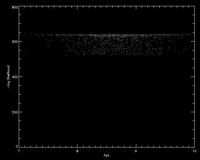
So our test point randomly explores the survey quality function (I'm not sure if what I used could be considered a likelihood function) acting like a atom exploring a potential energy function. Our test point starts hot, with a high probability of accepting even an unfavorable new point during its random walk. During the cooling timescale, it steadily calms its jumpy nature and hones in on a minimum.

Practical: To best understand the actual implementation, I will walk through the computing steps.

After receiving a starting point, it randomly permutes both the number of observations and the number of stars which would characterize a survey. Safety measures must be implemented to keep those parameters from exceeding possible bounds and ending the simulation.
In the beginning I imported an array of the magnitudes. Given the magnitudes of the brightest required number of stars, 60 hours of observing time, and each star needing to get the specific number of observations, the lowest instrument noise is calculated. Stellar jitter for each specific star is randomly pulled from a Gaussian centered at 15m/s with a standard deviation of 3 m/s. Stellar jitter and instrument error are added in quadrature.

Next, the parameters are sent into a survey function. 100 simulated surveys are run and the average number of planets discovered is returned. Within a survey, a star is randomly given a planet with a probability equal to .07 times its mass (the masses were also imported earlier on). The planet's properties are randomly selected from a distribution modeled on available data for intermediate mass stars. Each star receives n observations at times randomly pulled from the possible time vector. Three possible days exist per month over a 36 month period. "Observations" consist of calculating the radial velocity due to the planet and adding Gaussian jitter according to the noise. A planet is considered detected if the RMS of the observations is three times greater than the noise level.

Once back in the main simulation, the new set of parameters is kept if either

A. the number of planets produced is greater than that before
B. A uniformly randomly generated number is less than exp( - diff in planets/ Energy)

Hence at high energies, there exists a high chance of excepting the number, and at low energies the probability shrinks. I set the energy timescale to a decaying exponential according to advice on the internet. The energy starts at 20, and each step the energy decreases by 0.2%. I selected the numbers to start very jumpy and end very cold.

If the point is accepted, it is returned to a file.
This process is repeated 5000 times.

(And I just learned a good deal about making aesthetic graphs in MATLAB)

Why still a delta function PDF?

So...
Since the mass is still way too precise, I decided to move backward and look at the cluster fitting parameters. They turn out to be extremely precise too. Way too precise.

So, I went back and looked at the fitting paper that I read and I section that didn't make since before now makes since and I may be greatly wrong as to my process. They take the original isochrone, populate the HR diagram with many,many stars from this isochrone according to the initial mass function, and make a certain percentage of them unseen binaries according to some other distribution function. This creates a density on the HR diagram that is used to compute probabilities of a data point from that isochrone. Though the code would not be incredibly hard to write, it would be computationally difficult and greatly increase the time necessary for one cluster. Is that necessary and where I am going wrong?

Before I get too overwhelmed and confused, I think I'll try this on another cluster to compare results.

Better than a delta function PDF?

So I found an error in my code (I was dividing by the standard deviation in two separate places). The peak now does not move with a changing RMS.

And the error bounds are slightly better being twice as large, .002 solar masses instead of .001 ...

Survey Update
Stars:70
Clusters:24

All clusters with NGC# < 2287 have been completely rechecked for any hint of viability

Delta Function PDF?

So I am improving my cluster parameters fitting function, and creating my mass fittingfunction, and have a feeling something is wrong. All the code seems right. The cluster parameters returned visually fit the data well. The mass returned is within .1 of the rough distance only mass approximation. But the PDF for the mass is a delta function. I'm pretty sure we can't know the mass to a greater precision than .001 solar masses.

Later on, I have discovered that the PDF and even the maximum is highly dependent on the error. The RMS quoted for the star is .003, but MATLAB won't handle the extremely small probabilities that result from that. And obviously 67% of the bright stars are not .003 within a predicted isochrone. So I used .03, which gives the delta at 2.227, but I move it to .3, and it changes and moves the maximum to 2.5 (part of the loop that it obviously doesn't belong to).

I believe astrophysical properties, and not instrumentation, determine the majority of the error. Thus, I will fit all the clusters, and determine the error from tabulating the distribution of stars around their isochrones.

Note: I just eliminated fainter data since it included many background stars not even close to being on the main sequence, and I used CCD data.